I received questions from a couple of people asking me how I drew the network featured on the cover of PNAS (read about it here). Well, this blogpost is for you, and anybody else.

Before we get started we first need some data, go ahead and grab a small sample of the Copenhagen Network Study data from here — of course heavily anonymized. The csv-file is just a list of edges which denote that node i is connected to node j.

Before we start plotting stuff we first need to import some libraries. Note that I am using python 2.7 and, and at the time of writing, networkX version 1.11. If you have problems with importing the graphviz_layout package, please upgrade your pydot module to pydot2.

import matplotlib.pyplot as plt
import networkx as nx
import numpy as np
from networkx.drawing.nx_agraph import graphviz_layout

Then lets load some data.

edges = []
with open('edges_pnas_cover.csv') as f:
	next(f) # skip first line - header
	for line in f:
		edges.append(tuple(line.strip().split(',')))

Proceed by constructing an empty graph, populate it with the edge-data, and use NetworkX to position the edges nicely. For positioning nodes you can choose one of the many built-in algorithms in NetworkX, my favorite is graphviz, especially using the fdp or neato-layouts.

G = nx.Graph() # create empty graph
G.add_edges_from(edges) # populate it with edges

# layout graphs using graphviz
pos = graphviz_layout(G,prog="fdp")

Now we can already draw the network using nx.draw_networkx(...), but because we want the network to look nice we are not going to use networkX to draw the network (nothing personal against networkX). Instead we are going to use matplotlib.

plt.figure()

# draw edges
for ei,ej in G.edges():
	plt.plot([pos[ei][0],pos[ej][0]],[pos[ei][1],pos[ej][1]],'-',color='crimson',alpha=0.3,lw=0.8)

# draw nodes
# for n in G.nodes():
#	plt.plot(pos[n][0],pos[n][1],'o',color='crimson',markersize=2.5,markeredgecolor='#cccccc',markeredgewidth=0.1,clip_on=False)

plt.axis('off')
plt.savefig('pnas_cover_network.png',dpi=200,bbox_inches='tight')
plt.close()

This code produces something like the figure below. Note that I have not drawn the actual nodes, only links are shown. If, however, you are interested in the nodes as well you can draw them by commenting in the lines regarding nodes.

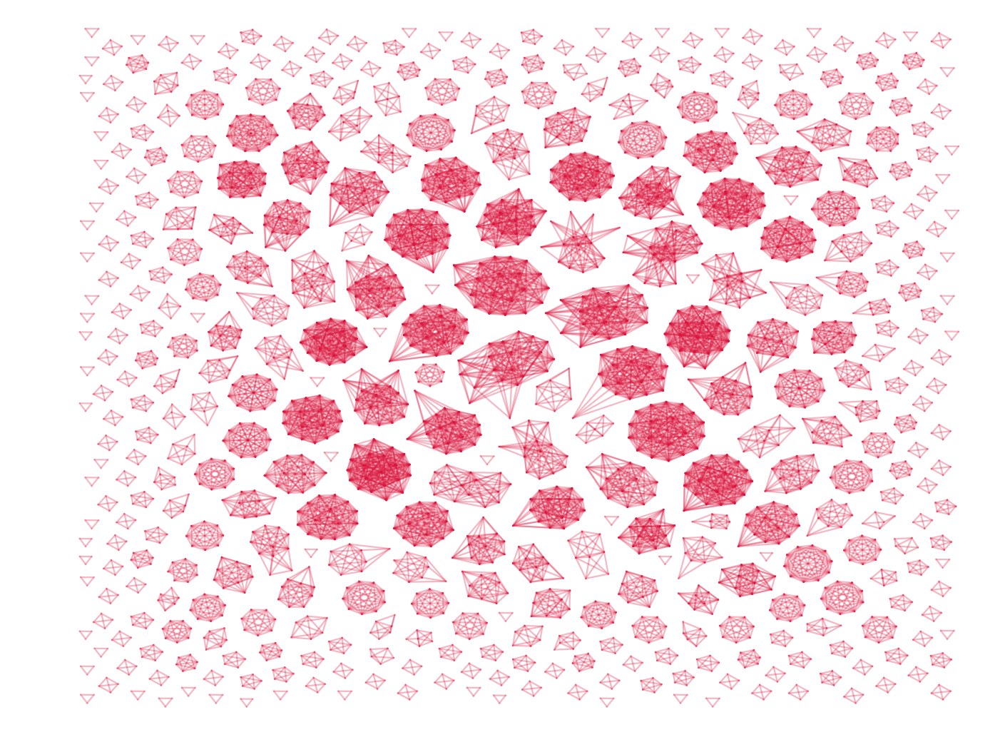
This look OK, but all edges have the same color and the figure is strangely elongated — we can do better then that. Lets color edges differently depending on their distance from a certain point, say from the bottom left. First we need to estimate the extend of the network, and calculate the minimal and maximal distance form all nodes to the reference point.

# find extent of network
x,y = zip(*pos.values())
min_x = min(x); max_x = max(x)
min_y = min(y); max_y = max(y)

# calculate distance from nodes to bottom left (min_x,min_y)
dist = dict([(n,np.sqrt((min_x-pos[n][0])**2 + (min_y-pos[n][1])**2 )) for n in G.nodes()])
min_d = int(min(dist.values())); max_d = int(max(dist.values()))

Notice we store the distance from each node to the reference point a dictionary named dist. [If you have a huge network with millions or even billions of nodes this might not be the best approach]. Now we are ready to assign a unique colors to each edge. Go ahead a select a colormap from matplotlib colors, or create your own custom colormap see here and here. I personally prefer viridis, but in this case we will use coolwarm.

For each distance unit we move away from the reference point we want the color of the edges/nodes to be slightly different. To achieve this we are going to create a dictionary named colors`` withmax_d - min_d + 1``` number of colors, basically this is the total number of distance units which we are going to distribute colors across. To separate colors evenly we use numpy’s linspace-function and to be able to reference colors we wrap it all into one big dictionary we use the zip function.

colors = dict(
		zip(
			range(min_d,max_d+1),
			plt.cm.coolwarm(np.linspace(0,1,max_d-min_d+1))
		)
	)

Now we can draw the network again using the following code:

plt.figure(figsize=(8.3,8.9)) # close to required size by PNAS (in inches)

# draw edges
for ei,ej in G.edges():
	dist_e = int(np.sqrt( (min_x - (pos[ei][0]+pos[ej][0])/2)**2 + (min_y - (pos[ei][1]+pos[ej][1])/2)**2))
	plt.plot([pos[ei][0],pos[ej][0]],[pos[ei][1],pos[ej][1]],'-',color=colors[dist_e],alpha=0.3,lw=0.5,clip_on=False)

# draw nodes
#for n in G.nodes():
#	plt.plot(pos[n][0],pos[n][1],'o',color=colors[int(dist[n])],markersize=2.5,markeredgecolor='#cccccc',markeredgewidth=0.1,clip_on=False)

# set axis
plt.xlim(min_x-1,max_x+1)
plt.ylim(max_y+1,min_y-1,)

plt.axis('off')
plt.savefig('pnas_cover_network_final.png',dpi=200,facecolor='black',bbox_inches='tight')
plt.close()

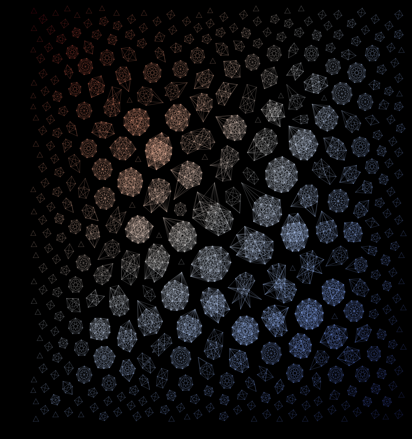
End result

Using a black background, our colormap, and the correct (PNAS) figure size. Congratulations! You can now use this code to draw your own versions of the network featured on the cover of PNAS. Maybe even do a startup where you print cool networks on t-shirts — I would definitely buy one.