Strange Attractors
 This Sunday while surfing the web I came across a figure depicting the Rössler attractor and while looking at it, it suddenly struck me that I have always seen it depicted from this specific angle. But what does it look like from other angles?
Curious, I sat down, quickly wrote a python script to generate the dynamics, used Matplotlib to plot the figure from multiple angles, and ffmpeg to aggregate them into an animation (see below).
One thing lead to another and soon I found myself reading about other strange attractors, such as Clifford attractors, and writing code to generate the figures you see above.
This Sunday while surfing the web I came across a figure depicting the Rössler attractor and while looking at it, it suddenly struck me that I have always seen it depicted from this specific angle. But what does it look like from other angles?
Curious, I sat down, quickly wrote a python script to generate the dynamics, used Matplotlib to plot the figure from multiple angles, and ffmpeg to aggregate them into an animation (see below).
One thing lead to another and soon I found myself reading about other strange attractors, such as Clifford attractors, and writing code to generate the figures you see above.
Below is a description of how I did it along with snippets of python code.
Rössler system
The Rössler system is given by the equations:
$$ \begin{align} \dot{x} = -y - z \\ \dot{y} = x + ay \\ \dot{z} = b + z(x-c) \end{align} $$which for certain parameter values of \(a\), \(b\) and \(c\) will exhibit chaotic behavior. I have chosen \((a,b,c) = (0.1,0.1,14)\). The following code simulates the dynamics for the system. First we import some packages and define the Rössler equations.
import numpy as np
import matplotlib.pyplot as plt
from mpl_toolkits.mplot3d import Axes3D

# define equation
def rossler_attractor(x, y, z, a=0.1, b=0.1, c=14):
	x_dot = - y - z
	y_dot = x + a*y
	z_dot = b + z*(x - c)

	return x_dot, y_dot, z_dot
Then we define some basic parameters such as how many steps we want to make and the size of each step.
# basic parameters
step_size = 0.01
steps = 100000

# initialize solutions arrays (+1 for initial conditions)
xx = np.empty((steps + 1))
yy = np.empty((steps + 1))
zz = np.empty((steps + 1))

# fill in initial conditions
xx[0], yy[0], zz[0] = (0.1, 0., 0.1)
It is possible to solve the equation system using scipy, but since this is a simple system we will just do it using numpy.
# solve equation system
for i in range(steps):
    # Calculate derivatives
    x_dot, y_dot, z_dot = rossler_attractor(x_s[i], y_s[i], z_s[i])

    xx[i + 1] = xx[i] + (x_dot * delta_t)
    yy[i + 1] = yy[i] + (y_dot * delta_t)
    zz[i + 1] = zz[i] + (z_dot * delta_t)
From here its easy to use matplotlib to plot the solution in 3D.
fig = plt.figure(figsize=(5,5))
ax = fig.gca(projection='3d')
plt.gca().patch.set_facecolor('black')

plt.plot(xx[:i], yy[:i], zz[:i],'-',color='white',lw=0.1)

# set limits
ax.set_xlim(-20,25)
ax.set_ylim(-25,20)
ax.set_zlim(0,50)

# remove ticks
ax.set_xticks([])
ax.set_yticks([])
ax.set_zticks([])

# make pane's have the same colors as background
ax.w_xaxis.set_pane_color((0.0, 0.0, 0.0, 1.0))
ax.w_yaxis.set_pane_color((0.0, 0.0, 0.0, 1.0))
ax.w_zaxis.set_pane_color((0.0, 0.0, 0.0, 1.0))

# set angle to view the figure from
ax.view_init(30, angle)

# save fig
plt.savefig('rossler.png', dpi = 300, pad_inches = 0, bbox_inches = 'tight')
plt.close()
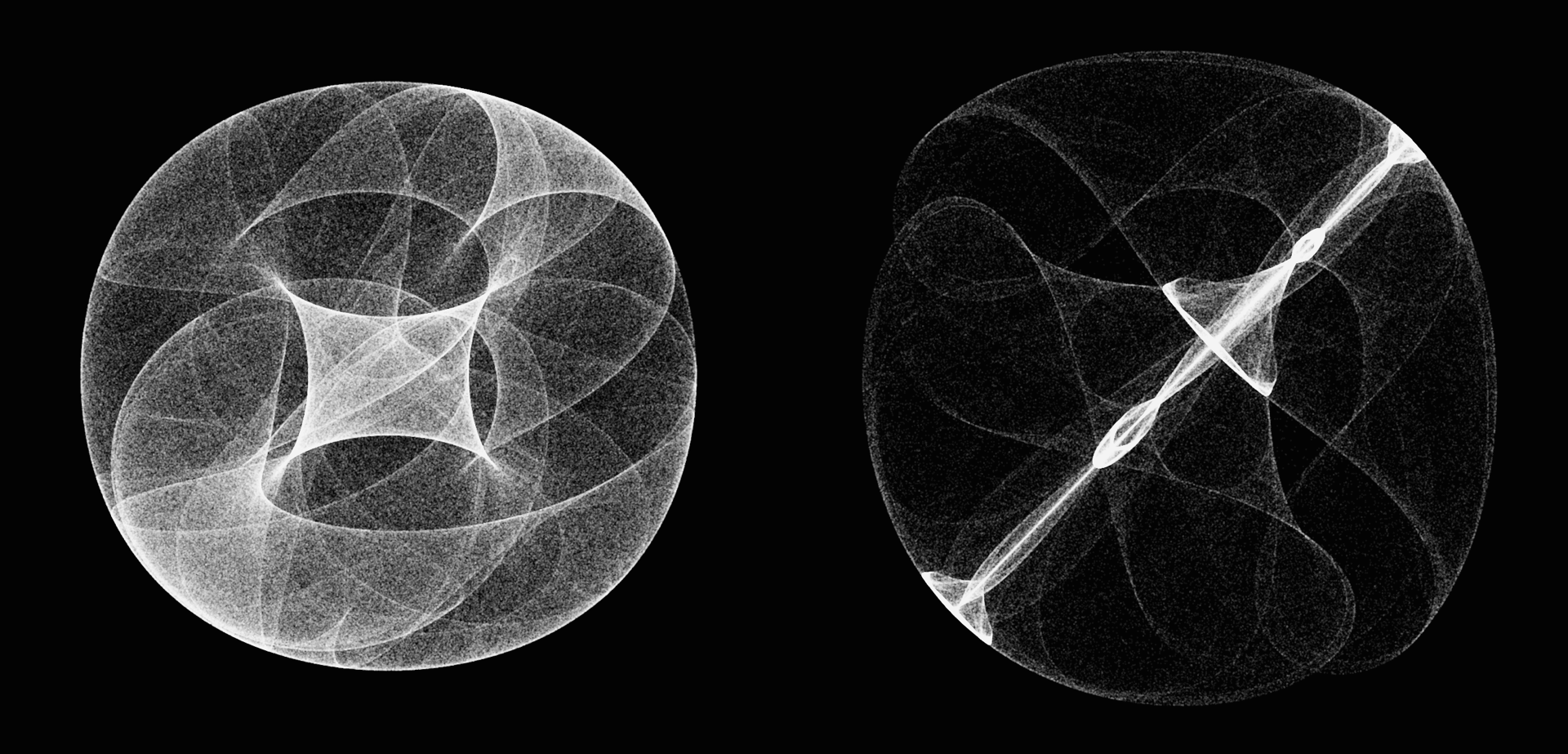
Clifford attractors
This is a peculiar form of attractor given by the 2D-equation system:
$$ \begin{align} x_{n+1} = \sin(ay_n) + c \cos(ax_n)\\ y_{n+1} = \sin(bx_n) + d \cos(by_n) \end{align} $$Again, for certain parameter values it exhibits chaotic behavior where it will abruptly jump around the state-space, so we are not going to plot the transitions as we did for the Rössler attractor. Instead we will only focus on the points it jumps to. The code is pretty similar to what we wrote above, so i wont go into detail.
import numpy as np
import matplotlib.pyplot as plt
import random

# define equation
def clifford_attractor(x, y, a=-1.4, b=1.6, c=1.0, d=0.7):
	x_n1 = np.sin(a*y) + c*np.cos(a*x)
	y_n1 = np.sin(b*x) + d*np.cos(b*y)

	return x_n1, y_n1

# basic parameters
steps = 1000000

# initialize solutions arrays (+1 for initial conditions)
xx = np.empty((steps + 1))
yy = np.empty((steps + 1))

# fill in initial conditions
xx[0], yy[0] = (0.1, -0.1)

# solve equation system
for i in range(steps):
	# Calculate derivatives
	x_dot, y_dot = clifford_attractor(x_s[i], y_s[i],a=a,b=b,c=c,d=d)
	xx[i + 1] = x_dot
	yy[i + 1] = y_dot

plt.figure(figsize=(5,5))
plt.plot(xx, yy,'.',color='white',alpha=0.2,markersize=0.2)
plt.axis('off')

plt.savefig('clifford.png', dpi = 300, pad_inches = 0, bbox_inches = 'tight',facecolor='black')
plt.close()
From here its just to run the script and generate some nice figures! The parameter values \((a,b,c,d) = (-1.4,1.6,1.0,0.7)\) generate the dynamics on far right attractor in the top figure.
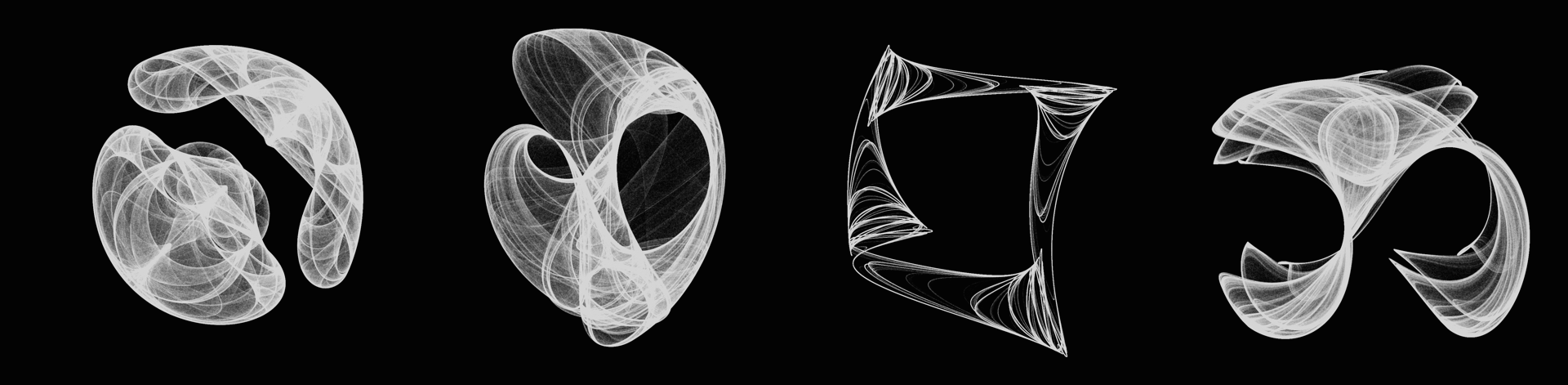
Trying other parameters yields amazing results!